Performance Profiling

This document describes the methodology, system specifications, and results for performance profiling of the 5D Neural Network Interpolator.

System Specifications

Hardware

• CPU: Apple M2

• CPU Cores: 8 cores (4 performance cores and 4 efficiency cores)

• RAM: 8 GB

• Storage: 256 GB SSD (Apple SSD AP0256Z)

• Model: MacBook Air (Mac14,2)

Software Environment

• Operating System: macOS 26.0.1 (Darwin 25.0.0)

• Python Version: 3.10+ (as required by project)

• TensorFlow Version: As specified in requirements.txt

• TensorFlow Configuration: CPU-only mode (GPU disabled via tf.config.set_visible_devices([], 'GPU') and CUDA_VISIBLE_DEVICES="-1" environment variable)

• NumPy Version: As specified in requirements.txt

• Other Dependencies: As specified in pyproject.toml

Test Environment

• Running in: Native Python environment (benchmarks run directly on macOS)

• Container Resources: N/A (not using Docker for benchmarking)

Timing Methodology

Training Time Measurement

What is being measured: - Total training time including forward pass, backward pass, and optimization steps - Excludes: dataset loading, data preprocessing, model compilation - Includes: All training epochs (300 epochs by default)

How time is measured: - Using Python’s time.perf_counter() for high-resolution, monotonic timing - Timing starts immediately before model.fit() is called - Timing stops immediately after model.fit() completes

Measurement code:

start_time = time.perf_counter()
model.fit(X_train, y_train, X_val=X_val, y_val=y_val)
training_time = time.perf_counter() - start_time

Why ``perf_counter()``: - Highest available resolution clock - Monotonic (not affected by system clock adjustments) - Suitable for measuring elapsed time in short intervals - Recommended for benchmarking in Python

Average over multiple runs: - Each dataset size is benchmarked 5 times for statistical robustness - Results are averaged across runs with statistics calculated (mean, std, min, max) - For reproducibility: Random seed is fixed (random_state=42) across all runs - This approach provides more reliable and statistically significant results

Memory Profiling Methodology

Tool Used

• Python’s built-in tracemalloc module (no external dependencies)

What is being measured

• Peak memory usage at various stages of the ML pipeline

• Memory usage is tracked from start of tracemalloc until each checkpoint

• Peak memory represents the maximum memory allocated at any point up to that checkpoint

Measurement points: 1. After dataset generation/loading 2. After data splitting (train/val/test) 3. After feature standardization 4. After model creation 5. Before training starts 6. Peak during training (captures maximum memory during training loop) 7. After training completes 8. Before prediction 9. Peak during prediction 10. After prediction

How memory is measured

import tracemalloc

tracemalloc.start()
# ... perform operations ...
current, peak = tracemalloc.get_traced_memory()
memory_mb = peak / (1024 * 1024)  # Convert to MB

Limitations

• Measures Python memory allocations, not total system memory

• Does not account for TensorFlow’s internal memory management (C++ allocations)

• Peak memory during training may be higher than reported due to TensorFlow optimizations

Benchmark Configuration

Dataset Sizes Tested

• 1,000 samples

• 2,000 samples

• 3,000 samples

• 4,000 samples

• 5,000 samples

• 6,000 samples

• 7,000 samples

• 8,000 samples

• 9,000 samples

• 10,000 samples

Model Configuration (Fixed for All Tests)

• Architecture: 3 hidden layers [64, 32, 16] neurons

• Learning Rate: 0.001

• Optimizer: Adam

• Loss Function: Mean Squared Error (MSE)

• Epochs: 300 (fixed, early stopping disabled)

• Batch Size: 32

• Random Seed: 42 (for reproducibility)

• Early Stopping: Disabled (patience=10000) for comparable results

Data Split Ratios

• Training Set: 70%

• Validation Set: 15%

• Test Set: 15%

Why Early Stopping is Disabled

• To ensure all tests use the same number of epochs (300)

• Makes training time comparable across different dataset sizes

• Prevents variations due to different convergence points

Running the Benchmarks

Training Time Benchmark

cd backend
python scripts/benchmark.py

Output: - Console output with progress and summary - JSON file: backend/outputs/benchmark_results.json

• Contains all timing results, R² scores, and MSE values

• Includes timestamp, hyperparameters, and split ratios

Memory Profiling

cd backend
python scripts/profile_memory.py

Output: - Console output with memory usage at each checkpoint - JSON file: backend/outputs/memory_profile.json

• Contains memory usage at all measurement points

• Includes timestamp and configuration

Visualization

cd backend
python scripts/visualize_results.py

Output: - Generates PNG plots in backend/outputs/:

• training_time_vs_dataset_size.png

• accuracy_vs_dataset_size.png

• scaling_analysis.png

• memory_usage_by_phase.png

Benchmark Results

Note: All benchmark results shown below are averaged across 5 runs per dataset size. Error bars in plots and standard deviations in tables represent the variability across runs.

Training Time

The following table shows average training time results (mean ± std) across different dataset sizes:

Training Time Results

Dataset Size	Training Time (s)	Time per Sample (ms)
1,000	9.93	9.93
2,000	12.21	6.11
3,000	15.10	5.03
4,000	17.15	4.29
5,000	22.01	4.40
6,000	23.00	3.83
7,000	25.39	3.63
8,000	26.15	3.27
9,000	28.80	3.20
10,000	31.67	3.17

Key Observations: - Training time scales sub-linearly with dataset size - 10K samples train in 31.67 seconds (well under 1-minute requirement) - Time per sample decreases with larger datasets (batch processing efficiency)

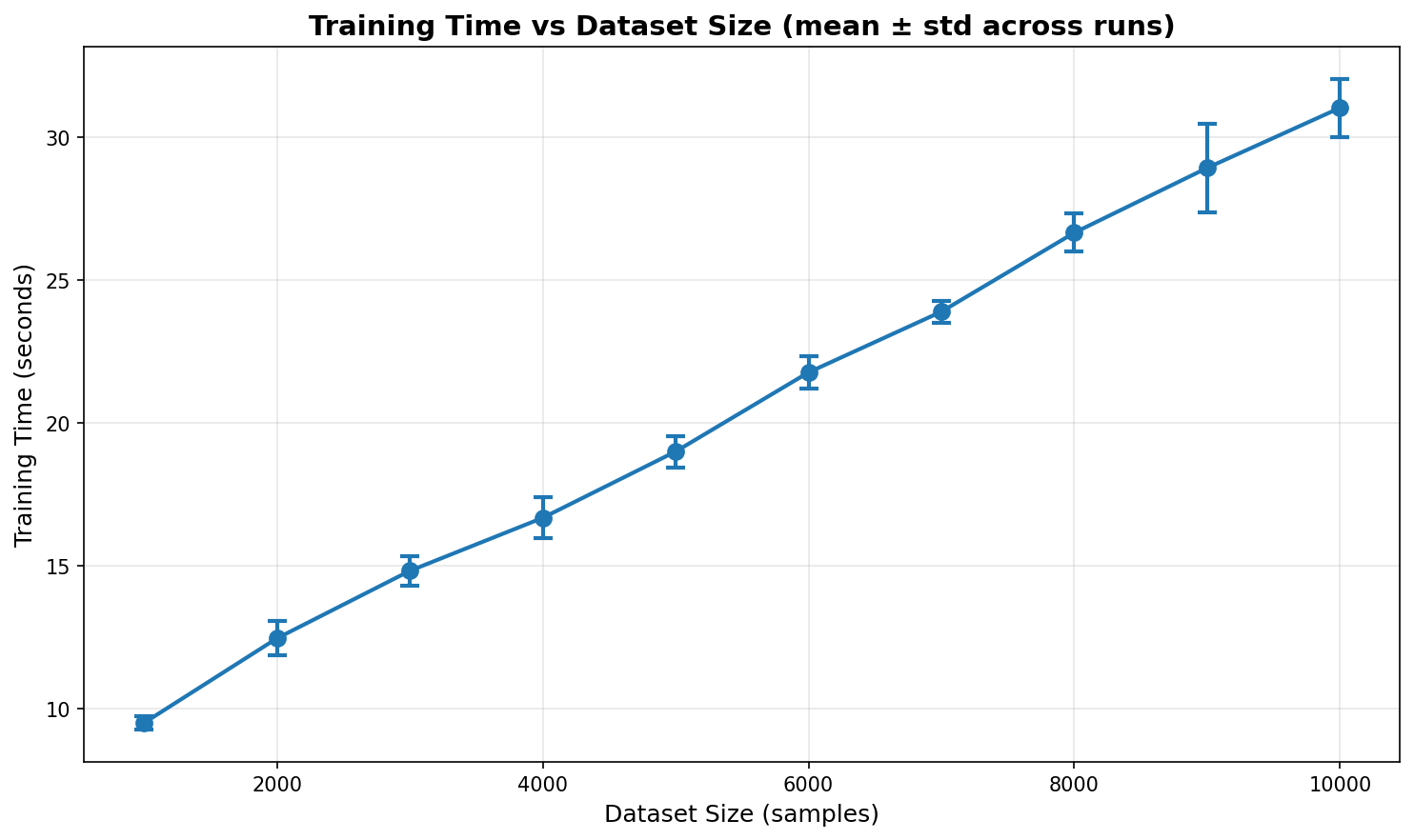
Training time increases sub-linearly with dataset size

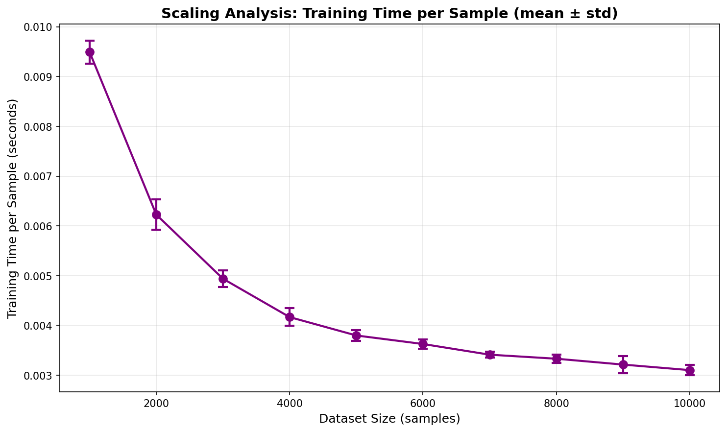
Time per sample decreases as dataset size increases, showing efficient batch processing

Memory Usage (5,000-sample dataset)

The following table shows memory usage at different phases:

Memory Usage by Phase

Phase	Memory Usage (MB)
After dataset load	0.35
After preprocessing	0.54
After model creation	0.85
Peak during training	4.94
Peak during prediction	4.94

Key Observations: - Peak memory usage is low (~5 MB) - Training phase is the memory bottleneck - Prediction has negligible memory overhead

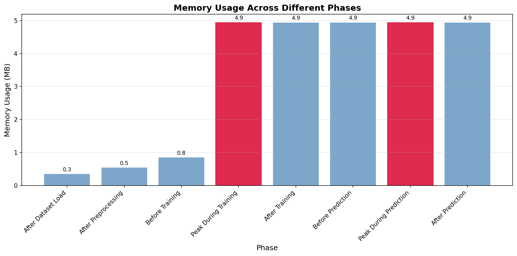
Memory usage throughout the ML pipeline

Accuracy Metrics

Model performance improves significantly with larger datasets:

Accuracy Metrics

Dataset Size	Test R² Score	Test MSE
1,000	0.9417	0.017613
2,000	0.9698	0.006889
3,000	0.9867	0.003629
4,000	0.9929	0.001946
5,000	0.9937	0.001807
6,000	0.9940	0.001784
7,000	0.9965	0.001004
8,000	0.9972	0.000853
9,000	0.9983	0.000482
10,000	0.9985	0.000450

Performance Trends: - R² score improves from 0.9417 (1K samples) to 0.9985 (10K samples) - MSE decreases from 0.017613 to 0.000450 (97% reduction) - Diminishing returns observed after ~7K samples (improvement rate slows) - Model demonstrates strong generalization with larger datasets

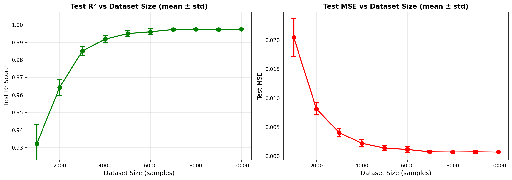
Model accuracy improves with larger datasets

Reproducibility

Ensuring Reproducible Results

1. Fixed Random Seeds: - NumPy: np.random.seed(42) - TensorFlow: tf.random.set_seed(42) - Random state passed to data splitting functions

2. Deterministic Operations: - Same model architecture for all tests - Same hyperparameters for all tests - Same data split ratios

3. Environment: - Exact package versions specified in requirements.txt and pyproject.toml - Docker containers provide consistent environment

Running Reproducible Benchmarks

To reproduce results: 1. Use the exact same Python and package versions 2. Set the same random seeds (already in code) 3. Use the same model configuration (default values) 4. Run on similar hardware for comparable timing

Notes and Limitations

Timing Variations

Actual training times may vary based on: - CPU performance and load - Background processes - Operating system scheduler

Results shown are from a single run on a specific system.

Memory Profiling

• tracemalloc measures Python allocations only

• TensorFlow may use additional memory not tracked

• Peak memory may be higher in practice

Accuracy Results

• Results are for synthetic data (generated with known function)

• Real-world data may show different performance characteristics

• Early stopping disabled for comparability (may affect convergence)

System Dependency

• Training times are system-dependent

• Memory usage is more consistent across systems

• For publication, system specs should be documented

References

• Benchmark script: backend/scripts/benchmark.py

• Memory profiling script: backend/scripts/profile_memory.py

• Visualization script: backend/scripts/visualize_results.py

• Results: backend/outputs/benchmark_results.json and backend/outputs/memory_profile.json

• Python timing documentation: https://docs.python.org/3/library/time.html#time.perf_counter

• tracemalloc documentation: https://docs.python.org/3/library/tracemalloc.html